Tool setup and run

To run correctly, the script requires proper setup according to the instructions below.

Download the latest stable version of the code as zip from here. Unzip it in your work directory, e.g. wd/rdl-tools/. The script has been developed to run as jupyter notebook. It has been tested on Windows10/11 but it can work on Linux and MacOS as well.

Python environment

• Python 3 needs to be installed on your system. We suggest the latest Anaconda distribution. Mamba is also supported.

• Create new rdl-tools environment from the provided rdl-tools.yml file. It can be done via Anaconda navigator interface (environments > Import ) or from the Anaconda cmd prompt:

  conda create --name rdl-tools --file <dir/rdl-tools.yml>`
  activate rdl-tools
  

Settings

Edit the .env file inside the notebook directories to specify your working directory:

# Environment variables for the CCDR Climate and Disasater Risk analysis notebooks

# Fill the below with the location of data files
# Use absolute paths with forward slashes ("/"), and keep the trailing slash
DATA_DIR = C:/Workdir/rdl-tools

Run Jupyter notebooks

• Navigate to your working directory: cd <Your work directory>

  cd C:/Workdir/rdl-tools
  

• Run the jupyter notebook.

  jupyter notebook GUI.ipynb
  

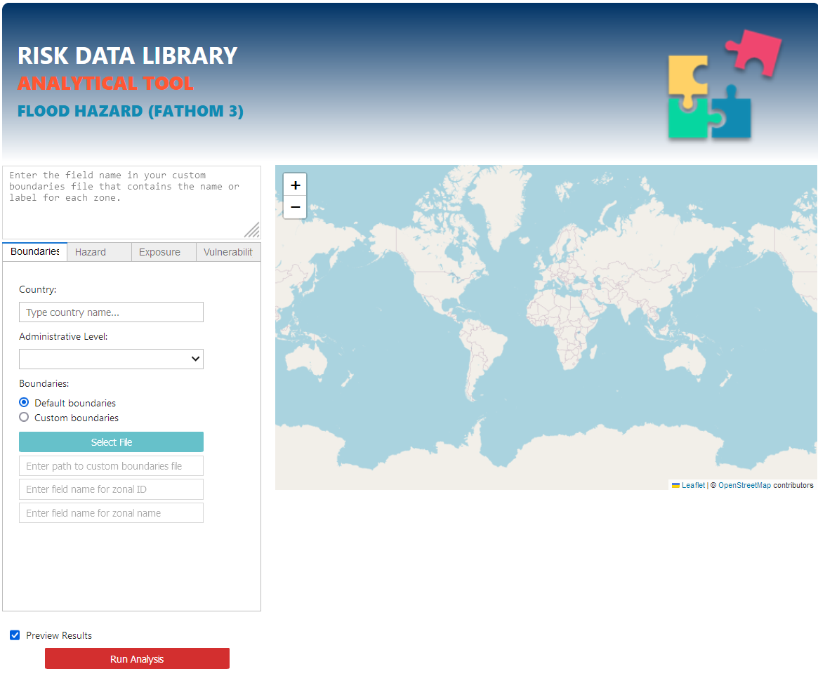
The main interface should pop up in your browser.

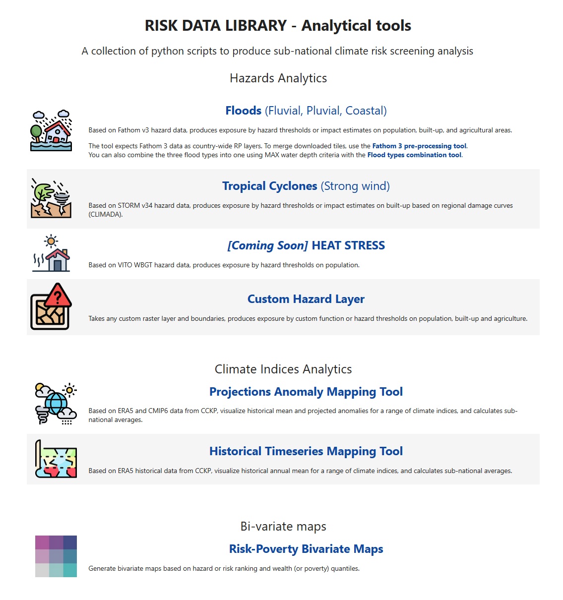
Select the hazard of interest to open the analytical notebook. E.g. for floods: