Flood Analytics#
The first notebook is dedicated to the screening of flood risk leveraging the Fathom v3 global model. Please refer to the instructions below to run the tool correctly.
Input data management#
The script fetches default data automatically. This includes:
National and sub-national boundaries from the WB ArcGIS repository.
Population data from WorldPop
Built-up data from WSF 2019
Land-cover (agriculture) data from ESA WorldCover
Default exposure datasets can be overridden by placing custom datasets in the EXP folder and pointing at those file in the interface.
The hazard data, when not automatically fetched, need to be downloaded and placed in the HZD folder; in case of tiled data, use pre-processing scripts to merge those into country-sized data. Each RP scenario is expected as a raster file (.tif) named as 1inyears.tif.
Example for Nepal, running analysis on undefended flood, 2020, RP100:
Work dir/
 - GUI.ipynb		Place the notebooks and related files in the main work directory
 - common.py
 - ...
 - Data/
   - HZD/NPL/FLUVIAL_UNDEFENDED/2020/1in100.tif	  	  Hazard layers
   - EXP/		                                  Exposure layers
   - RSK/		                                  Output directory
Caution
All spatial data must use the same CRS: EPSG 4326 (WGS 84)
Running the analysis#
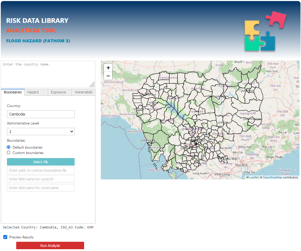
Select the country first. Sub-national boundaries for level 1 and 2 can be fetched automatically. Else, you can load custom boundaries as geopackage (WGS 84). You will need to specify the field to be used to run zonal statistics, and related label name (e.g. ADM3_PCODE and ADM3_EN).
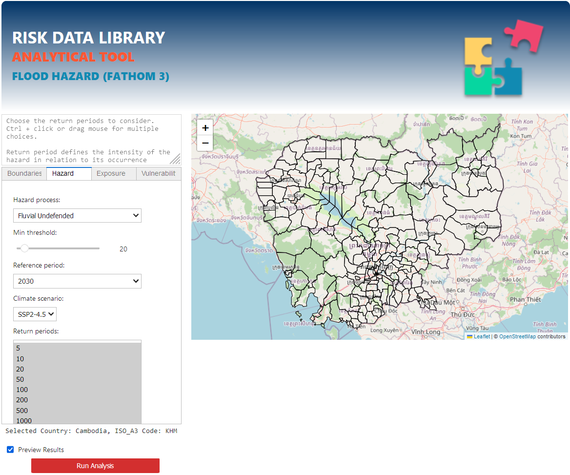
Move to Hazard tab: select the hazard process, the minimum hazard intensity threshold, the time period and climate scenario. Select one or more Return Periods (CTRL+Click / drag mouse).
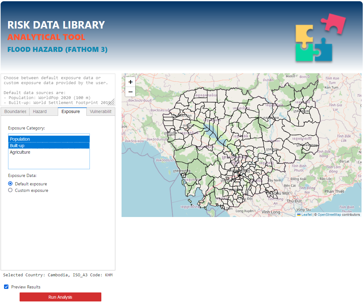
Select one or more Exposure categories (CTRL+Click / drag mouse). You can select a custom exposure layer for each selected category (.tif raster, WGS 84).
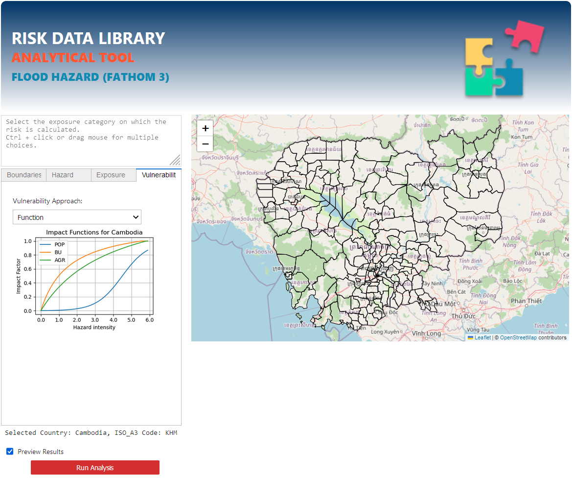
Select the approach to use for the analysis:
When using “function”, the best impact function is selected for the selected country and exposure categories.
When using “classes”, hazard intensity thresholds must be specified by the user.
Check “Preview results” to generate map and charts output in the GUI.
Manual Run#
Edit the manual_run.py file to specify:
country (
country):ISO3166_a3country codeflood hazard type (
haz_cat):'FLUVIAL_UNDEFENDED','FLUVIAL_DEFENDED','PLUVIAL_DEFENDED','COASTAL_UNDEFENDED','COASTAL_DEFENDED',hazard period (
period): the reference period of the hazard dataclimate scenario (
scenario): when future period, the associated climate scenario: ‘SSP1_2.6’, ‘SSP2_4.5’, ‘SSP3_7.0’, ‘SSP5_8.5’.return periods (
return_periods): list of return period scenarios as in the data, e.g.[5, 10, 20, 50, 75, 100, 200, 250, 500, 1000]exposure categories (
exp_cat_list): list of exposure categories:['POP', 'BU', 'AGR']exposure categories file name (
exp_nam_list): list of same length asexp_cat_listwith file names for exposure categories, e.g.:['GHS', 'WSF19', 'ESA20']If ‘None’, the default['POP', 'BU', 'AGR']applies
analysis approach (
analysis_app):['Classes', 'Function']If
'Function', you can set minimum hazard threshold value (min_haz_slider). Hazard value below this threshold will be ignoredIf
'Classes', you can set the number and value of thresholds to consider to split hazard intensity values into bins (class_edges)
admin level (
adm): specify which boundary level to use for results summary (must exist in theISOa3_ADM.gpkg file)save check (
save_check_raster): specify if you want to export intermediate rasters (greatly increases processing time)[True, False]
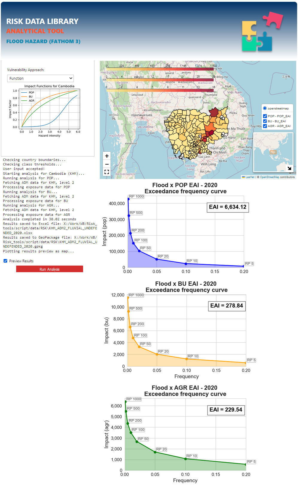
Example of manual_run.py running undefended river flood analysis (haz_cat) over Cambodia (country) over period 2020.
Include 10 return periods (return_periods) over three default exposure categories (exp_cat_list) using function approach; results summarised at ADM level 2 (adm). Do not save intermediate rasters (save_check_raster).
    # Defining the initial parameters - Example for function analysis
    country            = 'KHM'
    haz_cat            = 'FLUVIAL_UNDEFENDED'
    period	       = 2020
    scenario           = ''
    return_periods     = [5, 10, 20, 50, 75, 100, 200, 250, 500, 1000]
    min_haz_slider     = 20
    exp_cat_list       = ['POP', 'BU', 'AGR']
    exp_nam_list       = []
    adm_level          = 2
    analysis_app       = 'Function'
    # class_edges      = []
    save_check_raster  = False
Example of manual_run.py running defended coastal flood analysis (haz_cat) over Tunisia (country) over period 2030, scenario SSP2 - 4.5.
Include 5 return periods (return_periods) over three custom exposure categories (exp_cat_list) using hazard classes according to thresholds (class_edges); results summarised at ADM3 level (adm). Do not save intermediate rasters (save_check_raster).
    # Defining the initial parameters - Example for class analysis
    country            = 'TUN'
    haz_cat            = 'COASTAL_DEFENDED'
    period	       = 2030
    scenario           = 'SSP2-4.5'
    return_periods     = [10, 50, 100, 250, 500]
    min_haz_slider     = 0
    exp_cat_list       = ['POP', 'BU', 'AGR']
    exp_nam_list       = ['GHS', 'WSF19', 'ESA20']
    adm                = '3'
    analysis_app       = 'Classes'
    class_edges        = [50, 100, 150, 200, 250]
    save_check_raster  = False
After saving the file, to run the analysis:
$ python manual_run.py
The analysis runs on all selected exposure categories, in sequence. It will print a separate message for each iteration. In case of 3 exposure categories, it will take three iterations to get all results. The output is created as multi-tab .xlsx and multi-layer .gpkg. Depending on the power and number of cores on your CPU and the size and resolution of the data, the analysis can take from less than a minute to few minutes. E.g. for Bangladesh on a i9-12900KF (16 cores), 64 Gb RAM: below 100 seconds.