Hydro-Meteorological hazards#
Process or phenomenon of atmospheric, hydrological or oceanographic nature that may cause loss of life, injury or other health impacts, property damage, loss of livelihoods and services, social and economic disruption, or environmental damage (UNISDR).
Floods#
Flood hazard is commonly described in terms of flood frequency (multiple scenarios) and severity, which is measured in terms of water extent and related depth modelled over Digital Elevation Model (DEM). Flooding hazard can be triggered in different contexts. We can identify three main flood types:
Fluvial (or river) floods occur when intense precipitation or snow melt collects in a catchment, causing river(s) to exceed capacity, triggering the overflow, or breaching of barriers and causing the submersion of land, especially along the floodplains.
Pluvial (or surface water) floods are a consequence of heavy rainfall, but unrelated to the presence of water bodies. Fast accumulation of rainfall is due to reduced soil absorbing capacity or due to the saturation of the drainage infrastructures; meaning that the same event intensity can trigger very different risk outcomes depending on those parameters. For this reason, static hazard maps based on rainfall and DEM alone should be used with extreme caution. This is especially true for densely-populated urban areas, where the hazardous water cumulation is often the results of undersized or undermaintained discharge infrastructures.
Coastal floods (storm surge) occur when the level in a water body (sea, estuary) rises to engulf otherwise dry land. This happens mainly due to storm surges, triggered by tropical cyclones and/or strong winds pushing surface water inland. Like for inland floods, hazard intensity is measured using the water extent and associated depth.
The global Fathom model has consistently proven to be the best option for flood risk screening across WB projects. Fathom v3 is the latest release, improving the resolution to 30m and including additional features, such as coastal flooding and future climate projections.
Name |
||
|---|---|---|
Developer |
Fathom |
Fathom |
Version/Release |
v2 (2019) |
v3 (2023) |
Hazard process |
Fluvial flood, Pluvial flood |
Fluvial flood, Pluvial flood, Coastal flood |
Resolution |
90 m |
30 m |
Analysis type |
Probabilistic |
Probabilistic |
Frequency type |
Return Period (11 scenarios) |
Return Period (8 scenarios) |
Time reference |
Baseline (1989-2018) |
Baseline (1989-2018) |
Intensity metric |
Water depth [m] |
Water depth [m] |
License |
Commercial |
Commercial |
Other |
Includes defended/undefended option |
Includes defended/undefended option |
Notes |
Previous standard for WB analysis |
New standard for WB analysis |
See also
The Fathom v3 global dataset can be requested for use in World Bank projects by filling the request form.
When an open-access global dataset is preferred, there are a few alternatives that can be considered.
JRC flood hazard maps based on LISFLOOD model were recently updated. There are 7 probabilistic scenarios using 90 m resolution, those can be used for risk screening under current climate.
WRI “Aqueduct” flood hazard maps include both historical and future periods scenarios, using a resolution of 1 km.
UNEP/CDRI offers fluvial flood hazard maps as 9 return period scenarios under existing climate and long-term projected scenarios (SSP1 and SSP5) at 90 m resolution.
Name |
|||
|---|---|---|---|
Developer |
JRC |
WRI |
UNEP/CDRI |
Version/Release |
v2 (2024) |
v2 (2020) |
v1 (2023) |
Hazard process |
Fluvial flood |
Fluvial flood |
Fluvial flood |
Resolution |
90 m |
900 m |
90 m |
Analysis type |
Probabilistic |
Probabilistic |
Probabilistic |
Frequency type |
Return Period (7 scenarios) |
Return Period (10 scenarios) |
Return Period (9 scenarios) |
Time reference |
Baseline (1989-2020) |
Baseline (1960-1999) |
Baseline (2018) |
Intensity metric |
Water depth [m] |
Water depth [m] |
Water depth [m] |
License |
Open data |
Open data |
Open data |
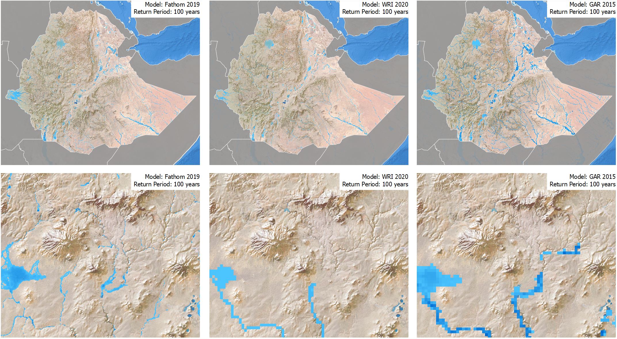
Fig. 13 Comparing modelled flood extent under historical scenario RP 100 years for a random location (Philippines): Fathom v3 2023 (left); Fathom v3 2023 (mid-left); JRC 2024 (mid-right) RWI - Aqueduct 2020 (right). Note how the Fathom model is able to better capture smaller discharge basins thanks to a better DTM resolution (30 m). Fathom 2 and JRC are comparable. The RWI data show its limitation at 1 km resolution.#
Coastal floods / Storm surge#
Regarding specific coastal flood and storm surge datasets, all models listed below include flood hazard simulations that account for the effect of Sea Level Rise under climate change projections: RWI uses CMIP5 climate data, while Deltares and UNEP-CDRI dataset is based on CMIP6. In addition to increasing water volumes, sea level projections account for land movements (sinking or rising land) caused by tectonic activity, large-scale underground extraction, or glacial isostatic adjustment.
WRI “Aqueduct” storm surge hazard maps include both historical and future periods scenarios, using a resolution of 1 km.
Deltares updated the WRI coastal flood model at 90 m, representing the best option in terms of resolution and time coverage (baseline + scenarios), and water routing, including inundation attenuation to generate more realistic flood extent.
UNEP/CDRI offers coastal flood hazard maps as 7 return period scenarios (10 to 1000 years) under existing climate and long-term projected scenarios (SSP1 and SSP5) at 90 m resolution.
Name |
|||
|---|---|---|---|
Developer |
WRI |
Deltares |
UNEP/CDRI |
Version/Release |
v2 (2020) |
v3 (2022) |
v1 (2023) |
Hazard process |
Coastal flood |
Coastal flood |
Coastal flood |
Resolution |
900 m |
90 m |
90 m |
Analysis type |
Probabilistic |
Probabilistic |
Probabilistic |
Frequency type |
Return Period (6 scenarios) |
Return Period (10 scenarios) |
Return Period (7 scenarios) |
Time reference |
Baseline (1960-1999) |
Baseline (2018) |
Baseline (1989-2020) |
Intensity metric |
Water depth [m] |
Water depth [m] |
Water depth [m] |
License |
Open data |
Open data |
Open data |
In addition to coastal flood projections, the NASA Sea Level Projection Tool allows users to visualize and download the sea level projection data from the IPCC 6th Assessment Report (AR6). The tool shows both global and regional sea level projections from 2020 to 2150, along with how these projections differ depending on future scenario or warming level. Data can be downloaded in multiple formats.
Landslides#
Landslides (mass movements) are affected by geological features (rock type and structure) and geomorphological setting (slope gradient). Landslides can be split into two categories depending on their trigger:
Dry mass movement (rockfalls, debris flows) is driven by gravity and can be triggered by seismic events, but they can also be a consequence of soil erosion and environmental degradation.
Wet mass movement can be triggered by heavy precipitation and flooding and are strongly affected by geological features (e.g. soil type and structure) and geomorphological settings (e.g., slope gradient). They do not typically include avalanches.
Landslide hazard description comes in form of deterministic susceptibility indices such as the NASA Landslide Hazard Susceptibility map (LHASA), the ARUP layer producded by GFDRR in 2019, and the most recent UNEP/CDRI layer, which improves the resolution to 90 m and offers both historical and future scenarios for the precipitation trigger. In addition, the Cooperative Open Online Landslide Repository (COOLR) reports on recorded landslide events, that can be used together with the susceptibility maps to validate their output.
Name |
|||
|---|---|---|---|
Developer |
NASA |
ARUP |
UNEP/CDRI |
Hazard process |
None |
Dry (seismic) mass movement |
Dry (seismic) mass movement |
Resolution |
1 km |
1 km |
100 m |
Analysis type |
Deterministic |
Deterministic |
Deterministic |
Frequency type |
none |
none |
none |
Time reference |
none |
Extreme rainfall: Baseline (1980-2018) |
Extreme rainfall: Baseline (1980-2018); Projections (2061-2100; SSP1, SSP5) |
Intensity metric |
Susceptibility index [-] |
Suscptibility-hazard index [-] |
Suscptibility-hazard index [-] |
License |
Open |
Open |
Open |
Notes |
Susceptibility obtained from land morphology variables |
Based on NASA landslide susceptibility layer, adding the hazard triggers |
Similar to ARUP, but improves on resolution and provides projections |
Fig. 14 ARUP landslide hazard layer. The qualitative index is displayed into 3 discrete classes (Low, Medium, High) according to thresholds set by ARUP (Low: <0.01; Moderate: 0.01-0.1; High: >0.1).#
Tropical cyclones#
Tropical cyclones (including hurricanes, typhoons) are events that can trigger different hazard processes at once such as strong winds, intense rainfall, extreme waves, and storm surges. In this category, we consider only the wind component of cyclone hazard, while other components (floods, storm surge) are typically considered separately.
Name |
|||
|---|---|---|---|
Developer |
NOAA |
NOAA |
TU Delft |
Version/Release |
2015 |
v4 (2024) |
v4 (2023) |
Hazard process |
Strong winds |
Strong winds |
Strong winds |
Resolution |
30 km |
10 km |
|
Analysis type |
Probabilistic |
Empirical |
Probabilistic |
Frequency type |
Return Period (5 scenarios) |
Return periods (10 to 10,000 years) |
|
Time reference |
Baseline (1989-2007) |
Baseline (1980-2022) |
Baseline (1984-2022) |
Intensity metric |
Wind gust speed [5-sec m/s] |
Many variables |
Wind speed, tracks |
License |
Open data |
Open data |
Open data |
The Global Assessment Report (2015) offered return period layers of max wind speed based on the first version of IBTrACS. These data have been superseded.
The latest version of IBTrACS (v4, 2024) can be leveraged to generate an updated wind-hazard layer, with better resolution and possibly the inclusion of orography effect. There are several attributes tied to each event; the map in figure below shows the USA_WIND variable (Maximum sustained wind speed in knots: 0 - 300 kts) as general intensity measure.
The STORM database has recently released their new version, which includes synthetic global maps of 1. maximum wind speeds for a fixed set of return periods; and 2. return periods for a fixed set of maximum wind speeds, at 10 km resolution over all ocean basins. In addition, it contains the same set for events occurring within 100 km from a selection of 18 coastal cities and another for events occurring within 100 km from the capital city of an island. The STORM dataset comes with projections as described in Bloemendaal, et al., 2022: those are generated by extracting the climate change signal from each of the four general circulation models listed below, and adding this signal to the historical data from IBTrACS. This new dataset is then used as input for STORM, and resembles future-climate (2015-2050; RCP8.5/SSP5) conditions. Both synthetic tracks and wind speed maps are available. These data can be used to calculate tropical cyclone risk in all (coastal) regions prone to tropical cyclones.
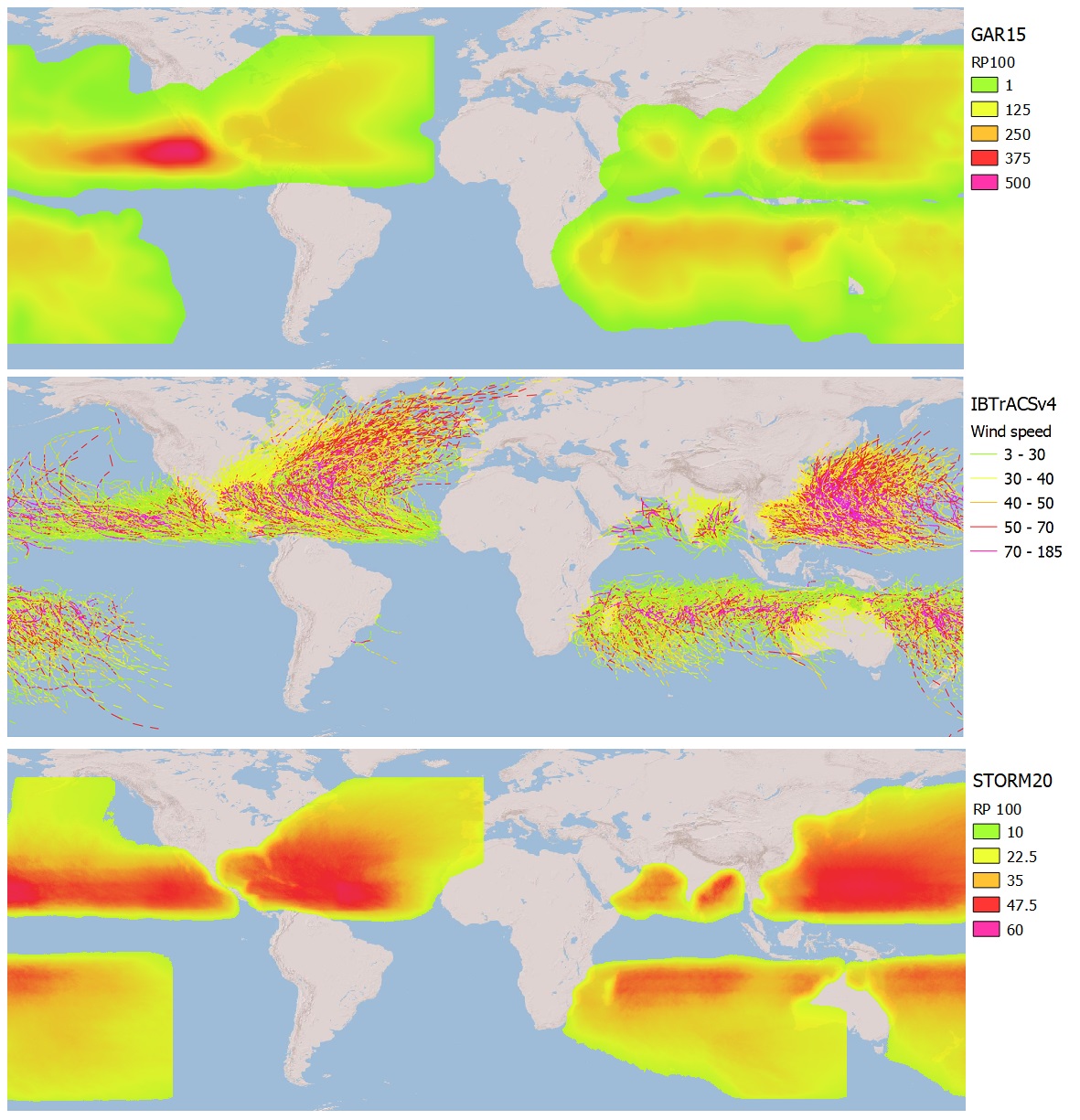
Fig. 15 Top: GAR 2015 cyclone max wind speed; Mid: IBTrACS v4 cyclone tracks; Bottom: STORMv4 synthetic cyclone tracks into max wind speed, RP 100 years.#
Drought & Water scarcity#
Drought hazard can be measured in different ways depending on the impact perspective.
To describe the overall hydrological balance of a region, the Standard Evapotranspiration-Precipitation Index (SPEI) or the self-calibrating Palmer Drought Severity Index (scPDSI) are often considered.
To describe water supply balance in terms of availability over demand, as well as other indices, the Water Risk Atlas produced by WRI Aqueduct provide an historical and future perspective.
To describe the observed agricultural impacts of droughts, the Agricultural Stress Index (ASI) produced by FAO depicts the frequency of severe drought affecting crop areas by means of remote-sensed Vegetation Health Index (VHI). FAO provides decadal, monthly and annual drought frequency over the period 1984-2024 split as the main crop season (S1) and secondary crop season (S2). For each season there are two indicators, according to two exposure intensity thresholds:
30 percent (1/3) of cropland area being affected by the drought event
50 percent (1/2) of cropland area being affected by the drought event
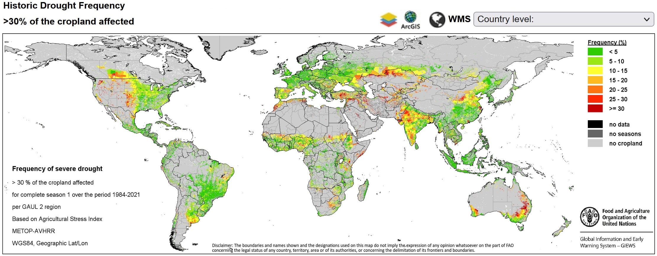
Fig. 16 FAO ASI global dataset showing historical drought frequency for >30% cropland area affected along the period 1984-2021.#
Heat stress#
Heat discomfort increases when hot temperatures are associated with high humidity [Coffel et al 2018]. Heat stress can cause long-term impairment and reduce labour productivity and incomes [Goodman et al 2018]. Extreme heat events lead to heat stress and can increase morbidity and mortality as well as losses of work productivity [Kjellstrom et al 2009, Singh et al 2015]. Not everyone reacts to the heat stresses in the same way, as individual responses are conditional on their medical condition, level of fitness, body weight, age, and economic situation [National Institute for Occupational Safety and Health 2016].
Various definitions regarding magnitude and duration thresholds and heat metrics exist. There are several heat indices involving both temperature and relative humidity, here are listed the most common ones: Wet-Bulb Globe Temperature (WBGT °C) and Universal Thermal Climate Index (UTCI °C). The two indices are similar and correlated, but while WBGT considers workload and overall effect on human health, UTCI is a more physically-based measure, thus it is easier to put it in relation to the physical measure of surface temperature (°C). It also has the advantage to consider cold stress extremes as well.
Name |
|||
|---|---|---|---|
Developer |
VITO |
Copernicus |
CORDEX |
Hazard process |
Extreme heat stress |
Heat stress on human health |
Extreme heat and humidity |
Resolution |
10 km |
30 km |
25 km |
Analysis type |
Probabilistic |
Index |
Probabilistic |
Frequency type |
Return Period (3 scenarios) |
None |
|
Time reference |
Baseline (1980-2009) |
Baseline (1979-2020) |
Baseline (1970-2000); Projections (2040-2070, 2070-2100) |
Intensity metric |
Wet Bulb Globe Temperature [°C] |
UTCI [°C] |
Heat Index, Humidex |
License |
Open data |
Open data |
Open data |
Notes |
Accounts for air temperature, humidity, wind speed, radiation, fatigue-heating. Includes intensity-impact classification. |
Accounts for air temperature, humidity. Includes intensity-impact classification. |
Wet-Bulb Globe Temperature (WBGT °C): the WBGT combines temperature and humidity, both critical components in determining heat stress. A probabilistic dataset (3 return periods: 5, 20 and 100 years) based on 1980-2009 data has been developed for the GFDRR by VITO and has since been used to measure heat stress in risk screenings and assessment. This layer is generally sufficient for country-level hazard screening, but it has several limitations for any hazard and risk assessment. Although downscaled to consider geomorphology and orography, the low grid resolution and relatively simple modelling makes it unfit to capture the heat island effect occurring in cities (Urban Heat Island) – nor the cooling effect of water bodies. That makes it unfit for any urban-scale assessment and generally sub-optimal for any sub-national assessment.
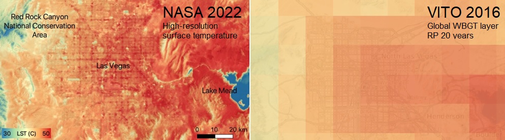
Fig. 17 Comparing recent high-resolution temperature maps showing the heat island effect in Las Vegas, and the presence of the lake; the global WBGT map based on global models resolution cannot capture these details.#
Universal Thermal Climate Index (UTCI °C): the UTCI is defined as the air temperature of a reference outdoor environment that would elicit in the human body the same physiological model’s response (sweat production, shivering, internal temperatures) as the actual environment. It is calculated based on near-surface air temperature, solar radiation, vapor pressure, and wind speed. For this specific dataset provided, the influence of solar radiation and wind speed is not considered and the UTCI is calculated from near-surface air temperature and vapor pressure solely, thus representing indoor or under-shade conditions.
In terms of future projections, both UTCI and WBGT projections have been produced under CMIP6 scenarios and are available via Copernicus CDS. The indices are provided for historical and future climate projections (SSP1-2.6, SSP2-4.5, SSP3-7.0, SSP5-8.5) included in the Coupled Model Intercomparison Project Phase 6 (CMIP6) and used in the 6th Assessment Report of the Intergovernmental Panel on Climate Change (IPCC). These have daily resolution and would allow to derive downscaled extreme temperature projections. These projections have not yet been processed into a frequency analysis, but that can be produced using the same approach.
Wildfire#
Wildfires are uncontrolled fires that spread through vegetation in rural and wildland-urban interface areas. Their frequency and severity are increasing due to climate change through higher temperatures, more frequent drought, and longer dry seasons. Wildfires can cause direct loss of life, destruction of infrastructure and vegetation, and severe air quality degradation.
Global probabilistic wildfire hazard datasets are available from several sources:
Name |
Developer |
Resolution |
Analysis type |
Time reference |
License |
|---|---|---|---|---|---|
EU-JRC |
0.1° |
Deterministic (fire weather index) |
Baseline + seasonal |
Open |
|
ESA CCI |
250 m |
Historical observations |
2001–2019 |
Open |
|
Knorr et al. |
0.5° |
Probabilistic |
Baseline + SSP1-2.6, SSP5-8.5 (2071–2100) |
Open |
Fire weather conditions — the key driver of wildfire hazard — can be characterised using the Fire Weather Index (FWI), which integrates temperature, humidity, wind speed, and precipitation into a single metric. CMIP6 projections of FWI are available through the Copernicus Climate Data Store and can be used to assess changes in wildfire hazard under future climate scenarios.