Baseline risk

Once required input layers have been created according to tool setup, the analysis can run.

• Select CCDR.ipynb and chose the hazard to analyse.

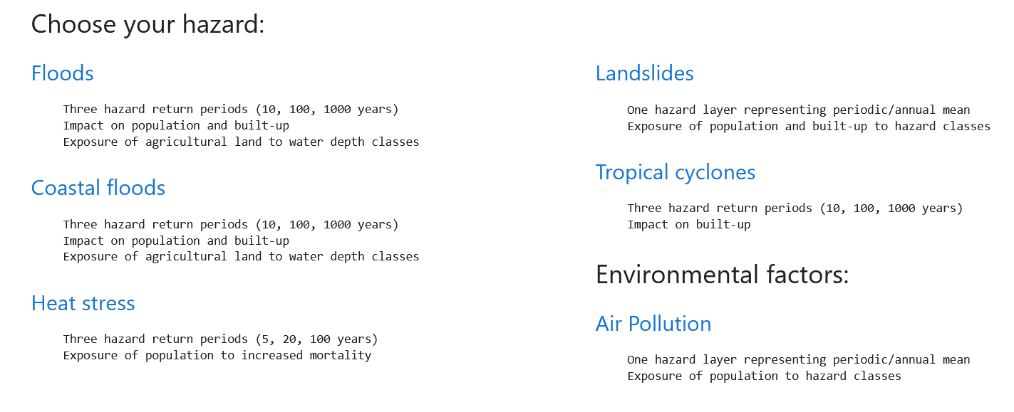
Fig. 46 Starting page for the CCDR python notebooks

• Execute all cells in the notebook (top bar > Cell > Run all). The last one will present the user interface. Select the country of interest, the exposure category and the level of administrative boundaries aggregation.

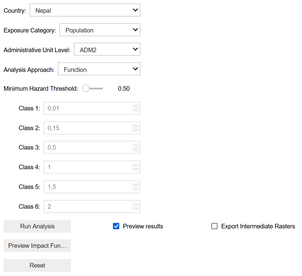
Fig. 47 Settings from one of the python notebooks

Note

Not all combinations of hazards x exposure are supported; some are not covered by appropriate damage functions or classification (read more). Select the analytical approach accordingly.

Analytical approach: Expected Annual Impact

This approach uses a mathematical relationship to calculate impact over exposed categories (read more). For example, flood hazard impact over population is calculated using a mortality function, while the impact over built-up uses a damage function for buildings.

The functions can be manually edited in the notebook, if a better model is available for the country of interest.

def damage_factor_builtup(x):
    """A polynomial fit to average damage across builtup land cover relative 
    to water depth in meters in Asia.

    The sectors are commercial, industry, transport, infrastructure and residential.

    Values are capped between 0 and 1, where water depth values >= 6m return a damage factor of 1

    References
    ----------
    .. [1] JRC, 2017
    """
    return np.maximum(0.0, np.minimum(1.0, -0.0028*x**3 + 0.0362*x**2 + 0.0095*x)) 	# Floods - AFRICA
    #return np.maximum(0.0, np.minimum(1.0, 0.9981236 - 0.9946279*np.exp(-1.711056*x))) # Floods - LAC
    #return np.maximum(0.0, np.minimum(1.0, 0.00723*x**3 - 0.1000*x**2 + 0.5060*x))	# Floods - ASIA

A minimum threshold can be set to ignore all values below - assuming that all risk is avoided under this threshold.

A chart of the impact function can be generated in the interface for the selected exposure category.

If you want to inspect all steps of the processing, you can select the option to export all by-products as tiff files:

• Export Intermediate rasters

Fig. 48 Click the button to start the processing

Once the analysis finishes, results are exported as geospatial data (.gpkg) and table (.csv).

By selecting:

• Preview results

A map will be generated at the end of the run, using a simple simbology.

Fig. 49 Example of output preview generated by the script: flood risk over built-up in Nepal

The map can be zoomed and inspected with the pointer to show all the values in the table.

Fig. 50 Example of output preview, subnational unit attributes as generated by the script: individual scenario exposure, impact and EAI summary

As explained in the risk concepts, EAI represents the aggregated absolute risk estimate:

• Fatalities [#] or mortality risk when considering impact over population;

• Hectars [ha] of built-up destroyed when considering impact over built-up.