Expected Annual Exposure (EAE)#
This analytical approach applies to probabilistic hazard scenarios (multiple layers by Return Period) which cannot be coupled with a proper physical vulnerability model, but can be ranked in terms of hazard intensity thresholds. Thus the hazard intensity layer is translated into discrete classes and, for each one, the total exposure for the selected category is calculated. For example, flood hazard over agriculture is measured in terms of hectars of land falling within different intervals of water depth.
This produces a mean estimate of Expected Annual Exposure (EAE) by hazard intensity classes for the historical baseline, as explained in the risk concepts. This is applied for:
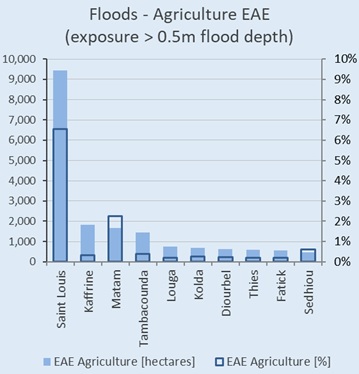
Floods: using water depth as hazard intensity measure, calculates agricultural land area affected by water detph over 0.5 meters.
Heat: using WBGT (°C) as hazard intensity measure, calculates the amount of population exposed to heat stress classes (strong, very strong, extreme).
Note
For example: there is no generalised impact model available for measuring flood impact over crops by means of water depth alone, because crop damage depends on a variety of additional factors, such as: duration of the submersion, water velocity, presence of pollutants, type of crop, stage of the crop cycle.
For this reason, following a rule of thumb, the risk metric chosen to measure flood risk over crops is simply exposure to water depth over 0.5 m.
SCRIPT OVERVIEW#
The python notebooks performs combination of hazard and exposure geodata from global datasets according to user input and settings, and returns a risk score in the form of Expected Annual Exposure (EAE) for baseline (reference period).
Note
A developer version (beta) of these scripts makes use of cpu parallelization.
User input is required to define country, exposure layer, and settings. Settings is used to define the classes thresholds. The script runs on one country and one hazard at time to keep the calculation time manageable.
The spatial information about hazard and exposure is combined at the grid level, using the horizontal resolution of the exposure layer (e.g. when using GHSL population layer, it is 100 meters). This is done for separate hazard intensity classes.
The exposure estimates by hazard are then summarised for the chosen administrative boundary (ADM) level using
zonal statistic. The expected annual exposure (EAE) is computed by multiplying the exposure value (for each hazard intensity class) with its exceedence frequency (1/RPi - 1/RPj) depending on the scenario. Theexceedance frequency curve (EFC)can be plotted. These outputs represent the core of the disaster risk historical baseline. The output is exported in form of tables, statistics, charts (excel format) and maps (geopackage).
DATA MANAGEMENT#
Download country boundaries for multiple administrative levels sourced from HDX or Geoboundaries. Note that oftern there are several versions for the same country, so be sure to use the most updated from official agencies (eg. United Nations). Verify that shapes, names and codes are consistent across different levels.
Download exposure data.
Download probabilistic hazard data, consisting of multiple RP scenarios.
SETUP THE NOTEBOOK#
Create environment and folder structure as explained in tool setup
Move verified input data into the tools folders
Use the interface to select the settings and start the processing; in particular, the number of classes and hazard thesholds to use.
PROCESSING#
LOOP over each hazard RPi layers:#
Classify hazard layer RPi according to settings: number and size of classes:
RPi->RPi_Cj(multiband raster)Each class
Cjof RPi is used to mask the Exposure layer ->RPi_Cj_Exp(multiband raster)Perform zonal statistic (SUM) for each ADMi unit over eac
RPi_Cj_Exp->table [ADMi_NAME;RPi_C1_Exp;RPi_C2_Exp;...RPi_Cj_Exp]
Example using 3 RP scenarios: (10-100-1000) and 4 classes (C1-4): `table [ADM2_NAME;RP10_C1_Exp;RP10_C2_Exp;RP10_C3_Exp;RP100_C1_Exp;RP100_C2_Exp;RP100_C3_Exp;RP1000_C1_Exp;RP1000_C2_Exp;RP1000_C3_Exp;RP1000_C4_Exp;]
Calculate EAE#
Calculate the exceedance frequency for each RPi ->
RPi_ef = (1/RPi - 1/RPi+1)whereRPi+1means the next RP in the serie. Example using 3 RP scenarios: RP 10, 100, and 1000 years. Then:RP10_ef = (1/10 - 1/100) = 0.09Multiply exposure for each scenario i and class j
(RPi_Cj_Exp)with its exceedence frequency(RPi_ef)->RPi_Cj_EAESum
RPi_Cj_Exp_EAEacross multiple RPi for the same class Cj ->table [ADMi;Cj_Exp_EAE]
Example using 4 classes (C1-4):table [ADMi;C1_EAE;C2_EAE;C3_EAE;C4_EAE]RP
Exc. frequency
C1_exp
C2_exp
C3_exp
C4_exp
C1_EAE
C2_EAE
C3_EAE
C4_EAE
10
0.09
4,036
1,535
2,111
1,967
363
138
190
177
100
0.009
8,212
5,766
5,007
13,282
739
519
451
1,195
1000
0.0009
8,399
5,134
4,371
25,989
756
462
393
2,339
Total
1,858
1,119
1,034
3,711
Perform zonal statistic of Tot_Exp using ADMi ->
[ADMi;ADMi_Exp;Exp_EAE]in order to calculateExp_EAE% = Exp_EAE/ADMi_Exp->[ADMi;ADMi_Exp;Exp_EAE;Exp_EAE%]
Present results#
Plot map of ADMi_EAI and related tables and charts to be included in reports and presentation. You can use open software QGIS to plot the geospatial data (.gpkg).
See also
More details on results presentation.